In almost all the examples of oscillations and waves dealt with on this site we have limited ourselves to analysing phenomena in the linear regime, although some non-linear or anharmonic effects have almost always been mentioned in the "further reading" of the various sections.

The main reason why we have not attempted a truly systematic treatment is that the effects of non-linearity are many and very diverse, and the physics of non-linear systems includes phenomena that are completely new compared with simple wave motion. Examples include:

• the emergence of chaotic dynamics, or of strange attractors
• the presence of new elementary excitations of the system that are not waves
• the interaction between waves (the superposition principle no longer holds)
• the modification of the behaviour of the normal modes of the system: they are no longer independent of each other, but coupled, and therefore no longer correspond to standing waves.
• the modification of the resonances and of the natural frequencies of the system
• the presence of hysteresis or saturation phenomena

etc.

Below we try to clarify the terms and give a single, but important, example.

Other examples, more complex but more interesting, can be found in the sections Fermi-Pasta-Ulam chain and modulational instability.

Linear and non-linear regime

Let us clarify the terms

• A single oscillator is in the linear regime when it is a harmonic oscillator, that is, when the restoring force is directly proportional to the distance of the oscillator from a point, which is its equilibrium point

${\displaystyle \mathbf {F} =-k(\mathbf {x} -\mathbf {x} _{0})}$.

This force therefore has a potential directly proportional to the square of the distance from the equilibrium point

${\displaystyle V={\frac {1}{2}}k(\mathbf {x} -\mathbf {x} _{0})^{2}}$.

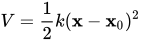
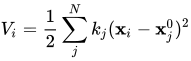
• A system of N oscillators is in the linear regime when each oscillator is subject to a set of harmonic forces. For example, the i-th oscillator will be subject to a total force equal to

${\displaystyle \mathbf {F} _{i}=-\sum _{j}^{N}k_{j}(\mathbf {x} _{i}-\mathbf {x} _{j}^{0})}$

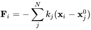
that is, to a potential

${\displaystyle V_{i}={\frac {1}{2}}\sum _{j}^{N}k_{j}(\mathbf {x} _{i}-\mathbf {x} _{j}^{0})^{2}}$

• Non-linear regime refers to all situations that depart from the previous case.

What happens in reality

• From the point of view of experimental reality, and without further assumptions, real physical systems must be considered all non-linear.
  • For example, real elastic forces do not follow Hooke's law for every displacement from the equilibrium position. This is easy to see by noting that an elastic system, as the deformation increases, first responds elastically, but then yields, remains permanently deformed, and finally breaks when stressed beyond a certain limit. All clearly non-linear phenomena.
  • From the mathematical-physics point of view, the presence of non-linear terms means that the forces are no longer simply directly proportional to the displacements, but also depend on their square, cube, etc. A typical example is an oscillator whose potential is

${\displaystyle V={\frac {1}{2}}k_{1}(\mathbf {x} -\mathbf {x} _{0})^{2}+{\frac {1}{3}}k_{2}(\mathbf {x} -\mathbf {x} _{0})^{3}}$.

• However, most physical systems can be considered approximately linear when the oscillations are small enough.
  • This property is equivalent to assuming that the forces (or potentials) can all be expanded in power series with a first-order term. Put simply, it is like saying "the Earth is flat for all practical purposes, as long as we look at a small enough portion of it".

The pendulum

It is extraordinarily easy to obtain complex behaviour even in apparently very simple systems. The ordinary pendulum is an example.

The equation of motion of the pendulum determines the time law of the oscillation angle. However, the net restoring force (due to the combination of the force of gravity and the tension of the string) depends on the sine of the oscillation angle. Therefore the exact equation of motion of the pendulum (keeping the other approximations: ideal massless string, point-like oscillating mass, motion in a plane) is

${\displaystyle \alpha +{\frac {g}{l}}\sin \theta =0}$,

(1)

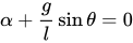
where α is the angular acceleration.

The common form, which reduces the pendulum to a harmonic oscillator, is actually the first-order approximation in the series expansion of the sine function

${\displaystyle \alpha +{\frac {g}{l}}\theta =0}$.

(2)

Using (2) instead of (1) gives the well-known expression for the period of the pendulum

${\displaystyle T=2\pi {\sqrt {\frac {l}{g}}}}$,

(3)

This law of motion agrees with Galileo's observation that the period does not depend on the amplitude of the oscillation, but only equation (1) also describes large-amplitude oscillations correctly. For these oscillations the period is given by

${\displaystyle T=2\pi {\sqrt {\frac {l}{g}}}\left(1+{\frac {1}{4}}\sin ^{2}{\frac {\theta _{max}}{2}}+{\frac {9}{64}}\sin ^{4}{\frac {\theta _{max}}{2}}+\cdots \right)}$.

(4)

The following figures show that oscillations of larger amplitude have a longer period than those of smaller amplitude. Moreover, their shape is no longer sinusoidal.

Oscillations of 15° and 150° compared. The period of the wider oscillation is much longer than that of the smaller one.	Angular velocity-angle diagram (phase space) for an oscillation of 15°. The sinusoidal oscillation generates an ellipse (Lissajous figure).	Angular velocity-angle diagram (phase space) for an oscillation of 150°. The oscillation is not sinusoidal, and therefore does not generate a Lissajous figure.

The Van der Pol oscillator

A model type of non-linear oscillator with several practical applications is the Van der Pol oscillator. It satisfies the equation

${\displaystyle {\dot {\omega }}+\theta +\mu (\theta ^{2}-1)\omega =0}$

where ${\displaystyle \omega ={\dot {\theta }}}$ and ${\displaystyle \alpha ={\dot {\omega }}}$ are the (angular) velocity and acceleration of the oscillator respectively.

The first two terms describe a harmonic oscillator of period ${\displaystyle 2\pi \;}$, since the proportionality constant between angular acceleration and angle has magnitude 1; the last term is responsible for the non-linear behaviour. Let us see how.

Graphical analysis

To get an idea of the properties of this oscillator, we solved the Van der Pol equation numerically and represented the motion in two ways in the following figures. The first column shows the usual law of motion, in which the oscillation angle is plotted as a function of time. The second column instead shows the angular velocity as a function of the angle. This representation (called phase space) has several advantages over the traditional one. In particular, it makes it easy to see whether there are limit cycles, or attractors, towards which the motion of the system is attracted from different initial conditions.

As a reference, we have drawn the trajectory of the Van der Pol oscillator in black, and that of the harmonic oscillator with the same initial conditions in red.

Let us now examine the plots. A further brief analysis is given in the next section.

• For the chosen initial condition, the amplitude of the oscillations always increases gradually until it reaches a limit cycle
• The shape of the limit cycle does not depend on the initial conditions, but only on the value of the parameter ${\displaystyle \mu }$, and departs further from the harmonic cycle (a circle) the larger the value of ${\displaystyle \mu }$.

	Law of motion	Phase space
${\displaystyle \mu =0.1}$
${\displaystyle \mu =0.5}$
${\displaystyle \mu =1}$
${\displaystyle \mu =4}$

The following observation suggests that the oscillator is robust with respect to the initial conditions. Indeed, we see that a limit cycle exists whether we start the motion inside or outside it. In other words, if the initial oscillations are too small they will be amplified, while if they are too large they will be damped down to a stable value. The limit cycle reached is the same in both cases.

${\displaystyle \mu =1.5}$	Law of motion	Phase space
${\displaystyle \theta (0)=30^{\circ };\omega (0)=1}$
${\displaystyle \theta (0)=-80^{\circ };\omega (0)=2}$

Further details

Let us see how we can justify the previous observations starting from an analysis of the equation of motion. Recall that the only non-linear term is the one proportional to ${\displaystyle \mu }$. Examining the equation

${\displaystyle {\dot {\omega }}+\theta +\mu (\theta ^{2}-1)\omega =0}$

we see that

• if ${\displaystyle \mu =0}$ the oscillator clearly reduces to a harmonic oscillator. Its motion will be purely sinusoidal, and the angle-velocity diagram will follow a circular trajectory. In the images above these lines are shown in red as a reference.
• if ${\displaystyle \mu >0}$ the added term has two effects that compensate each other:
  • for oscillations beyond a certain limit angle (in this case ${\displaystyle |\theta |>1}$) the term is positive, and corresponds to removing energy from the oscillator. Essentially it is equivalent to a friction term proportional to the velocity of the motion. In essence, it says that large-amplitude oscillations tend to be damped
  • for oscillations below the limit angle (in this case ${\displaystyle |\theta |<1}$) the term is negative, and corresponds to adding energy to the oscillator. Essentially it is equivalent to an external force proportional to the velocity of the motion. Adding energy means that small-amplitude oscillations tend to be increased.

We can see that the net effect of the non-linear term, whatever the initial conditions, is to stabilise the oscillations on a limit cycle, which is the point of balance between oscillations that are too large, which tend to be damped, and small oscillations, which instead tend to grow in amplitude. The shape of the limit cycle will depart further from the circle (harmonic oscillator) the larger the value of ${\displaystyle \mu }$.